September 1, 2025

Samarth Rawat
Founding Engineer
Understanding Cold Starts
When a deployment experiences a traffic spike, it needs to scale up by launching new instances. The delay between a new container being created and it becoming ready to serve traffic is known as the “cold start time.” Minimizing this delay is essential for maintaining a responsive and scalable application.For all examples in this post, we’ll be using the
meta-llama/Llama-3.1-8B-Instruct model running on L40S GPUs to provide concrete performance numbers.What happens during a cold start?
During a cold start, a series of sequential events occur. At a high level, it looks like this:- A new instance is created.
- Model Loading
- The model is downloaded into storage.
- The model weights are loaded into GPU memory.
- Torch.compile
- Dynamo bytecode transformation
- Graph compilation
- Graph capture
- Init Engine
Optimizing the vLLM Workflow in Kubernetes
Kubernetes deployments are ephemeral, meaning each new pod starts from a clean slate. This can be inefficient for ML models, as many time-consuming initialization steps are repeated unnecessarily. By identifying and caching the outputs of these steps, we can dramatically reduce startup times. Let’s break down the process layer by layer to see where we can introduce optimizations.1. Model Loading
Model Downloading
First, the model’s weights must be available on the instance’s local storage. You have two primary options:-
Download from Hugging Face on startup:
- Pros: No additional infrastructure cost.
- Cons: Slow and unreliable. Download speed is limited by the node’s network bandwidth and is dependent on Hugging Face’s availability.
-
Cache the model in a volume:
- Pros: Much faster and more reliable, especially for instances with lower network bandwidth. Eliminates dependency on Hugging Face during scaling.
- Cons: Incurs storage and data transfer costs.
The storage cost is$0.30/GB-monthand the data transfer cost is$0.03/GB. For example, caching a 16GB model that cold starts 40 times a month would cost approximately $24.
Weight Loading
After the model is downloaded, its weights must be loaded into GPU memory. This process can be a significant bottleneck. You can optimize this step by using specialized loaders via theload_format parameter in vLLM, including extensions like fastsafetensors or run-ai. You can find the list of supported formats in the vLLM documentation.
2. Torch.compile
torch.compile is a just-in-time (JIT) compiler that dramatically speeds up model execution at runtime. However, this performance comes at the cost of an initial compilation step that takes about 52 seconds for our example model.
Fortunately, torch.compile includes a built-in caching system. In a Kubernetes environment, you can persist this cache by using a shared volume. The first pod will perform the compilation and save the cache, making it instantly available to all subsequent pods.
3. Graph Capture
To minimize kernel launch overhead, vLLM uses CUDA Graphs to capture the entire model execution flow. By default, this process captures a wide range of batch sizes and takes approximately 54 seconds. You can significantly reduce this time by tailoring the graph capture to your specific request patterns. For example, if your service primarily handles smaller batches, you can instruct vLLM to only capture graphs for those sizes.4. Init Engine
The final step is initializing the vLLM engine, which involves loading the model, compiled kernels, and captured graphs. This process also benefits from its own caching layers, like theflashinfer cache.
Case Study: Putting It All Together
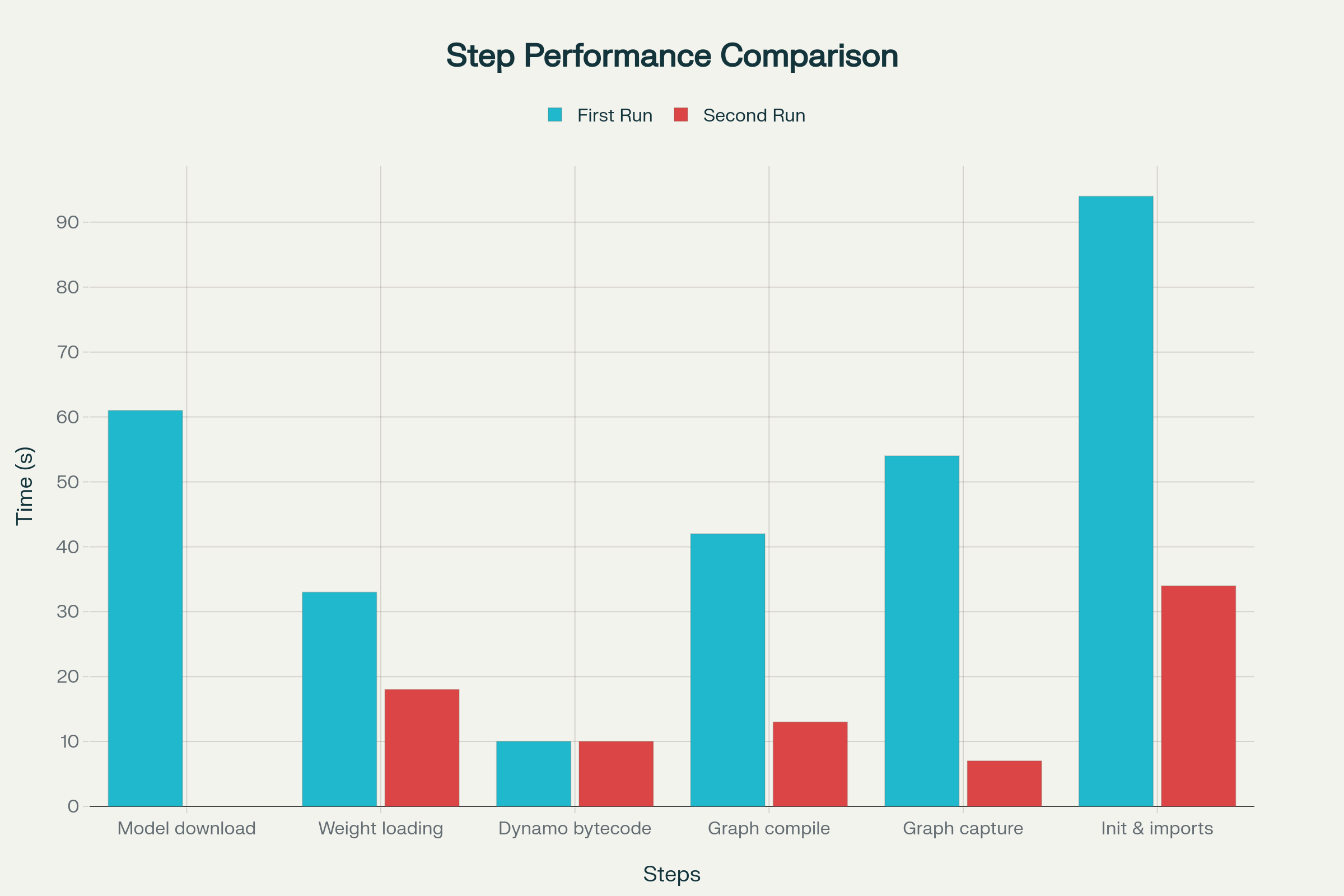
Let’s see what this looks like in practice.The Baseline: Before Optimization
Here is the initial cold start time for our Llama 3.1 8B model, with each step running from scratch:
Total Time: 294 seconds (4 minutes, 54 seconds)
The Solution: Caching and Optimization
We can dramatically improve this by implementing two key changes:- Use a cached volume: We’ll use Tensorkube to mount a persistent volume at
/root/.cache. This will cache the model download,torch.compileresults, and other initialization artifacts. - Optimize graph capture: We’ll limit the CUDA graph capture to the batch sizes relevant to our workload (
1, 2, 4, 8, 16, 24, 32, 64).
The Result: After Optimization
With these changes, the cold start performance is drastically improved:
Total Time: 82 seconds (1 minute, 22 seconds)
By caching the model and optimizing graph capture, we reduced the cold start time by over 70%, from 294 seconds down to 82 seconds.
Practical Implementation: Dockerfiles & Configuration
Now that we’ve seen the impact of these optimizations, let’s look at how to implement them in practice.Choosing Your Strategy: To Cache or Not To Cache?
The decision to cache your model on a volume versus downloading it on startup depends on a trade-off between cost, reliability, and performance. You should cache your model when:- Reliability is critical. Caching eliminates a dependency on external services like Hugging Face, which could be unavailable.
- Your instance has limited network bandwidth. For GPUs without guaranteed high-speed networking (e.g., “up to 20 Gbps”), a cached volume will almost always be faster.
- You are using a relatively small model. For smaller models, the monthly storage cost is often negligible compared to the performance gains.
- Cost is a primary concern. Downloading on demand avoids storage costs.
- Your instance has guaranteed high-speed networking. Machines with 15-25 Gbps or more of guaranteed bandwidth can often download models faster than they can read from a network-attached volume.
Example Dockerfiles
Here are two example Dockerfiles that showcase both approaches.We are mounting our efs volume at
/root/.cache in both these cases.GPU Architecture Reference
You need to set theTORCH_CUDA_ARCH_LIST environment variable to match the compute capability of your target GPU. This ensures torch.compile generates the most optimized code. Here’s a quick reference for supported AWS instances:
If you are having trouble finding the
Network Bandwidth for your GPU, please scroll down until you find the Product details table and scroll to the right.